Computing Asymmetric Curves with 5PL and 4PL
Five Parameter Logistic and Four Parameter Logistic Curve Fitting of Asymmetric Assays
Use of the five parameter logistic (5PL) function to fit dose response data can significantly improve the accuracy of asymmetric assays over the use of symmetric models such as the four parameter logistic (4PL) function. This is especially important for ELISA tests (enzyme-linked immunosorbent assays) whose dose response curves are more asymmetric than earlier types of assays. Asymmetry is also a characteristic trait with bioassay curves. An accurately weighted 5PL can extend the usable dose range of the curve an order of magnitude beyond that of an unweighted 4PL. STATLIA MATRIX uses powerful numeric algorithms plus accurate weighting with the test’s historical data to provide the gold standard for 5PL curve fitting in analysis software. (For more information, see the Tech Note: Comparing 4PL and 5PL Curve Fitting Models and Optimizing Calibrator Doses.)
Weighting and Residuals
Statistical curve fitting uses a method called least squares regression fitting. Least squares regression derives the one set of coefficients that has the smallest sum of squared residuals (RSSE, or residual sum of squares error) for that curve model. A weighted squared residual is the vertical distance between the observed point and the curve, squared, divided by the estimated variance at that point. The estimated variance is obtained from a distribution of responses at specific concentrations. Initial variance estimates can be made from one assay, and more reliable variance estimates can be obtained from a pool of 6 or more historical assays. This distribution of responses is approximately normal for most immunoassay and bioassay data.
Critical to obtaining the best curve fit are the estimated variances used to compute the weighted squared residual at each point. Because immunoassay and bioassay data are quite heteroscedastic (unequal variances), each response is weighted by the inverse of the estimated variance of that response:
weighti = 1/estimated variancei
It is common for the variances of points at the high-response end of a curve to be three or four orders of magnitude larger than variances of points at the low response end. The reaction kinetics of the assay are also a major factor in the response variances of each dose, and the reaction kinetics vary widely between different tests. Weighting the squared residual errors with the estimated variances at each point allows the responses from the noisier and less noisy points to contribute equally to the regression curve. This produces the most accurate concentration estimates. Sample concentrations computed from unweighted curve fitting procedures can differ from properly weighted curves by hundreds of percent. See Tech Note: Curve Weighting for more information.
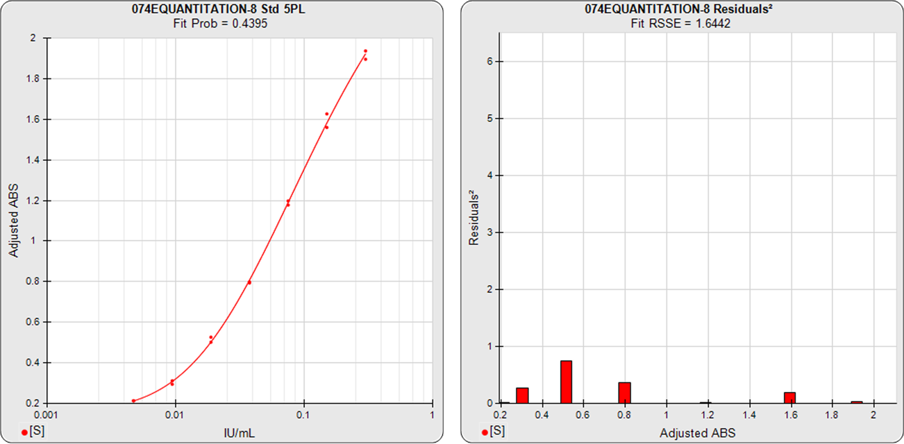
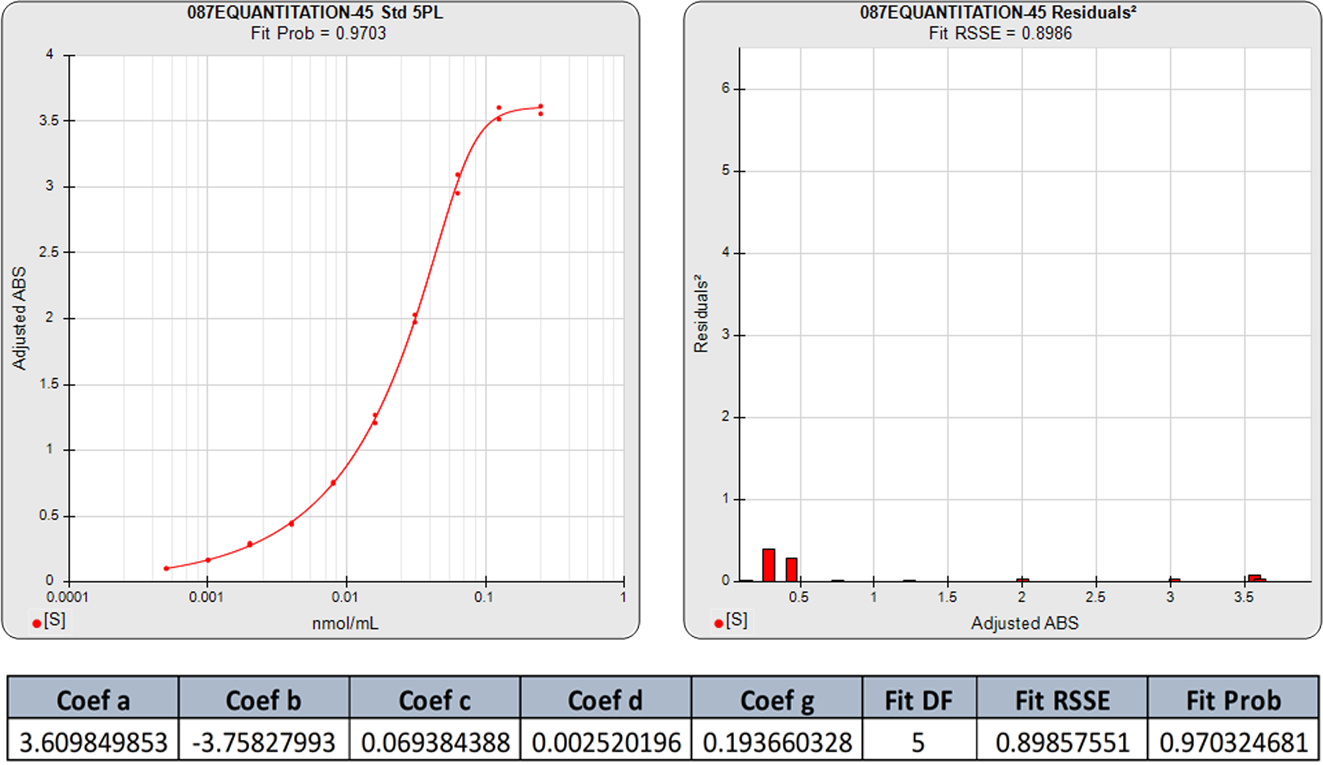
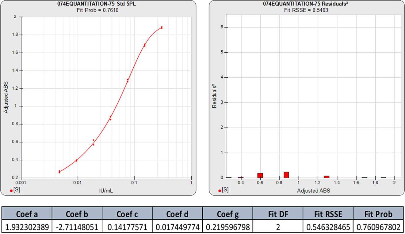
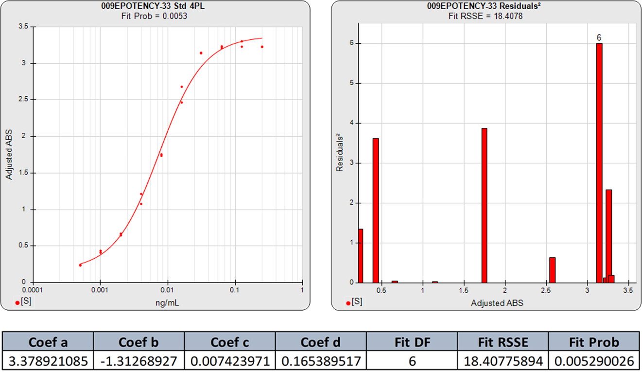
The standard curve graph on the far left shows the 5PL dose response curve from an ELISA assay. The graph to its right shows the weighted squared residual errors (red bars) between the observed responses and predicted responses off the curve divided by the estimated variance for each dilution of that curve.
The average RSSE from a pool of regression curves should equal the degrees of freedom (number of points – number of curve coefficients) when the residuals are accurately weighted. For each individual curve regression, the residuals2 of each dilution should vary randomly in magnitude.
The residual2 of each dilution should be low. A single high residual2 indicates a bad dilution. Many high residuals2 indicates a bad curve fit.
.
Describing the 5PL Curve
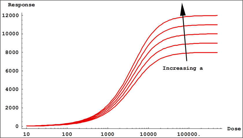
The equations for the 5PL and 4PL curve models are:
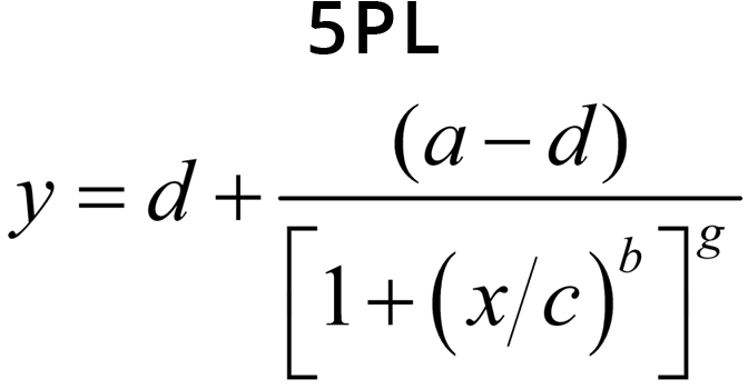
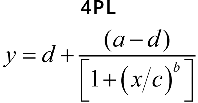
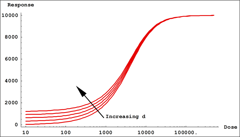
- Coefficients a and d control the location of the upper and the lower asymptotes of the equation. These are the values that the responses ( y ) approach as the log of the dose ( x ) approach 0 and infinity.
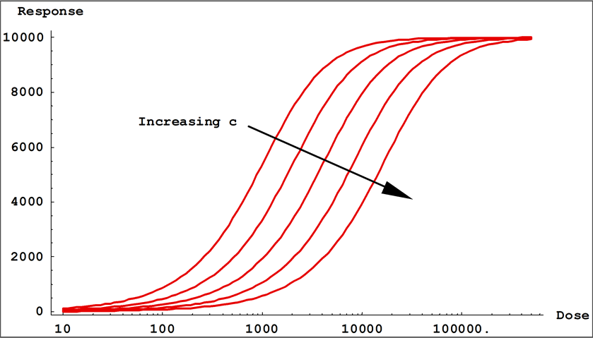
- Coefficient c controls the location of the transition on the dose ( x ) axis. This is the inflection point in the transition between the two asymptotes.
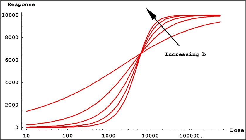
- Coefficient b is the slope at the transition point ( c ) and controls the rate of approach to the asymptotes. The sign of b controls whether the curve is monotonically ascending or descending.
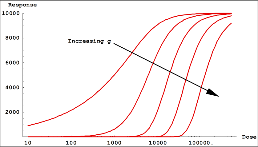
- Coefficient g controls the asymmetry in a 5PL curve. This is the difference in the rates of approach from the inflection point ( c ) to the lower and the upper asymptotes. In a 4PL curve, g = 1 and is factored out.
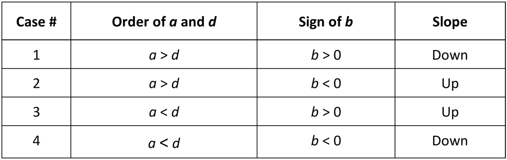
The relationship between the order of a and d, the sign of b, and the slope of the monotonic 5PL and 4PL functions can be seen in the 4 cases above. Note that when g = 1 and the curve is actually a 4PL curve, two pairs of the cases can be combined into single cases. For 4PL curves, case #1 and case #4 or case #2 and case #3 generate the same functional forms, and both conventions are used in the industry. For 5PL curves, all 4 cases produce distinct functional forms.
Small values of | b | result in a gradual transition from one asymptotic region to the other, while large values of | b | result in fast transitions. In 5PL curves, when a > d, b controls the rate of approach to the upper asymptote a, while the product ( b * g ) controls the approach to the lower asymptote d. If g < 1, the curve will approach the upper asymptote faster than the lower asymptote and c will be located closer to the upper asymptote than to the lower asymptote. The opposite is true when g > 1. This is all reversed when a < d. In 4PL curves where g = 1, the curve passes through the midpoint between the asymptotes at x = c and y = (a + d) / 2.
The sensitivity of the best fit coefficients are influenced by three factors: the number of data points; the location of the data points; and the intrinsic sensitivity of the coefficients to small changes in the shape of the curve. This last is especially noticeable in the 5PL curve. The coefficients b, g, and c are coupled, so large changes in their respective values can be traded off so that the nature of the transition between the asymptotes is altered. The changes in the transition region include such effects as sharpening or smoothing the “knee” at the beginning and end of the transition zones and changing the length and steepness of the transition. The lack of datapoints in the asymptotes, the upper or lower shoulder regions of the curve, or the transition region can result in wide ranges of values for the relevant coefficients. This is because without a datapoint in the region to constrain the RSSE, the fitting algorithm can trade off large coefficient changes for subtle improvements in the shape. The 4PL does not have any coupled coefficients, and both ends are constrained by the shape of the other end.
It is important to note that the 5PL and 4PL logistic models are mathematical shape functions only; their coefficients do not correlate with any physical properties of the immunoassay or bioassay reaction. This has been extensively discussed in the literature. This can also be demonstrated with a set of competitive binding assays, each having a maximum baseline sample (0 dose standard) and a minimum baseline sample (nsb). Calculate the mean of the baseline samples and the mean of the a and d coefficients from the assay set. Then match whether the observed baseline samples and equivalent coefficients of each assay are both greater than or less than their respective means. The lack of correlation between the baseline samples and their analogous coefficients demonstrates that the logistic asymptotes are just shaping parameters to fit the observed data points and are not valid estimates of maximum and minimum responses.
Evaluating Curve Fits
According to regression statistics literature, the RSSE from an accurately weighted regression of normally distributed data will be approximately chi-square distributed with number of points minus number of coefficients degrees of freedom. This can be shown as follows:
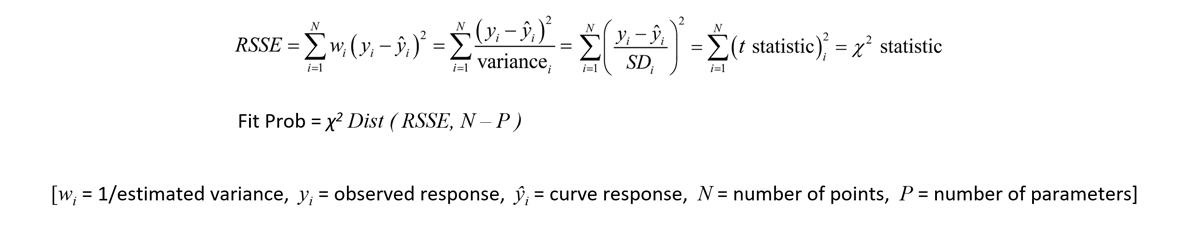
In statistics, one of the most common ways to determine how well a candidate curve is fitting the true curve is to determine how likely (probable) it is for the candidate curve to have yielded the observed data under the assumption that the candidate curve is actually the true curve. The best fitting curve (MLE) is therefore the curve most likely to have given rise to the observed data. The fit probability is that likelihood, and it applies to any 5PL, 4PL or linear regression fit. The fit probability (Fit Prob) is a statistical measure of how well a curve fits a set of data. The Fit Prob applies equally well to fits of single logistic curves used in ELISA as well as to the unconstrained and constrained logistic curves used in potency assays . The number of data points and coefficients determine the degrees of freedom, so the least parameterized model that best fits the data will have the highest probability. Since probabilities offer a familiar scale that is independent of the curve model or number of data points, the Fit Prob obtained from an accurately weighted least squares regression model is the ideal measure for goodness of fit.
Comparing 5PL and 4PL Curve Fits
The 4PL logistic curve has been used extensively in immunoassay and bioassay data reduction. One reason for this is that the process of fitting the 5PL function is difficult for many data reduction software programs, with the result that the 4PL function has continued to be used even for highly asymmetric data. Even when the 5PL is offered, many software programs revert to a 4PL when they are unable to compute a 5PL fit. However, the advanced numerical algorithms plus the accurate weighting estimates used in STATLIA MATRIX ensure that even the most asymmetric and ill-behaved curve data are easily computed with a reliable 5PL fit.
5PL
4PL
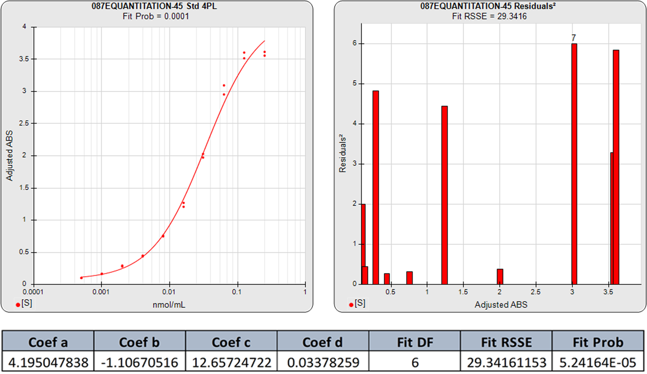
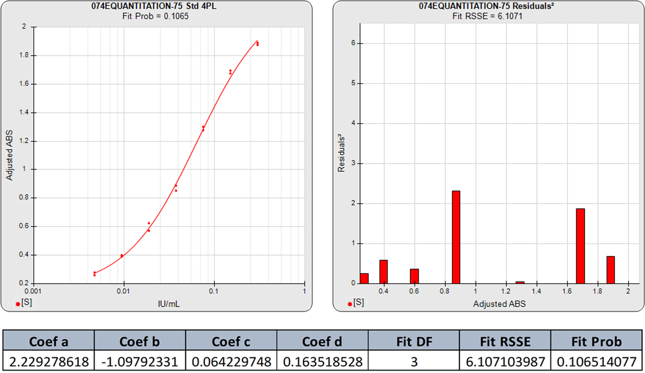
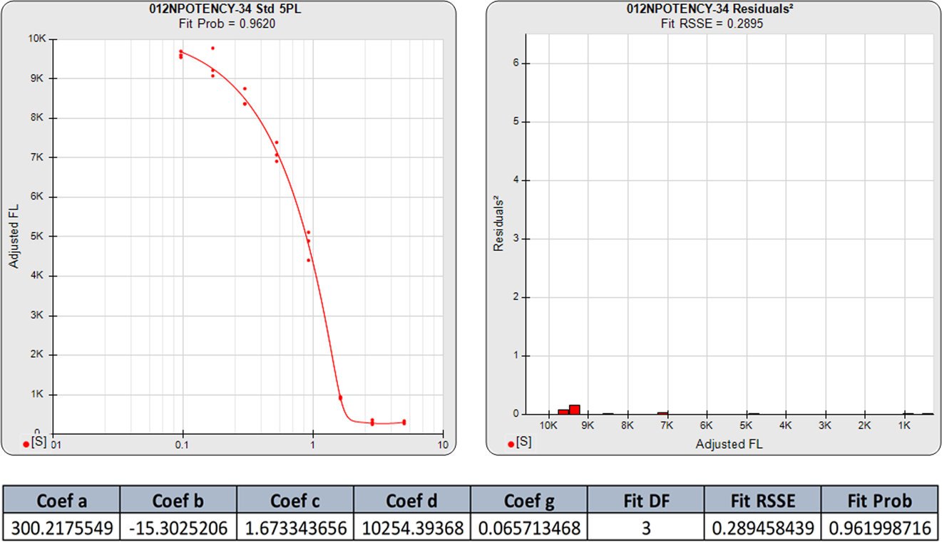
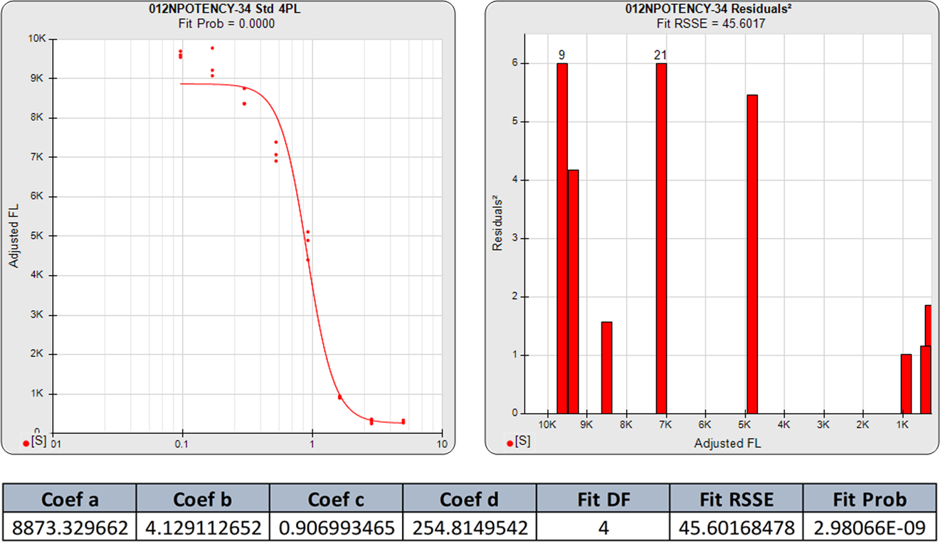
The 5PL curve and dilution weighted squared residuals (left two graphs) and the 4PL curve and dilution weighted squared residuals (right two graphs) above were computed using the same data and the same weighting estimates. The sharp transition at the upper asymptote and the more gradual transition to the lower asymptote is typical for ELISA assays. Because the curve is accurately weighted at each point, the lack of fit of the 4PL curve is the same at both ends of this asymmetric curve. However, scaling effects in semi-log standard curve graphs always make the low end appear to be a better fit than it actually is compared to the high end. But since the weighted residual graphs are the same scale for all dilutions, and each dilution response is weighted with its own estimated variance, the nature of the lack of fit of the 4PL is clear. This example shows why an appropriately weighted 5PL can extend the usable range of asymmetric curves up to an order of magnitude in sensitivity over a 4PL.
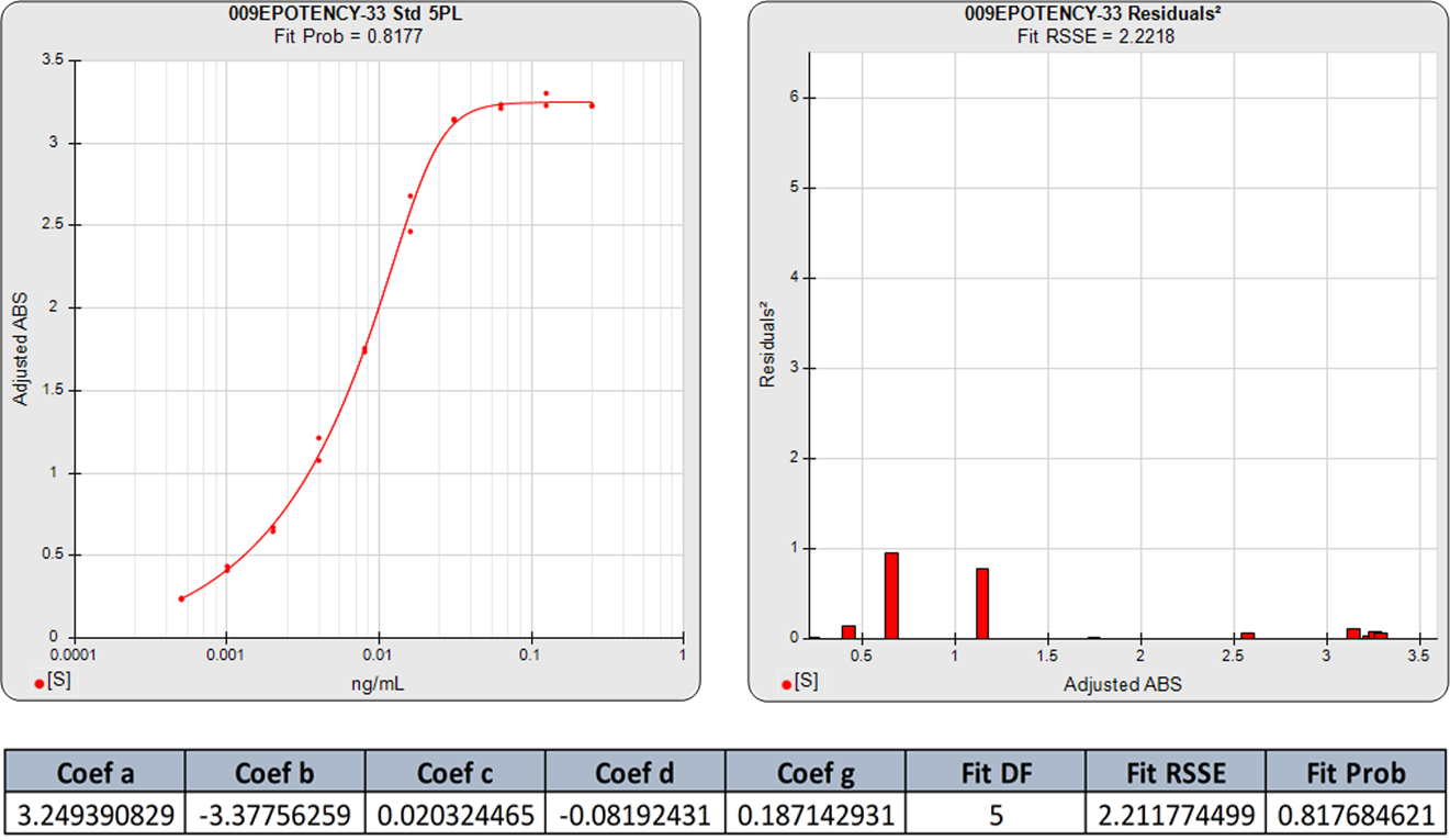
The graphs below show the improvement in the 5PL fit over the 4PL of even fairly symmetric data points. Although this 4PL is an acceptable curve fit, the 5PL curve is a substantially better fit. This is because all immunoassay and bioassay curves with sigmoidal shapes have some asymmetry.
5PL
4PL
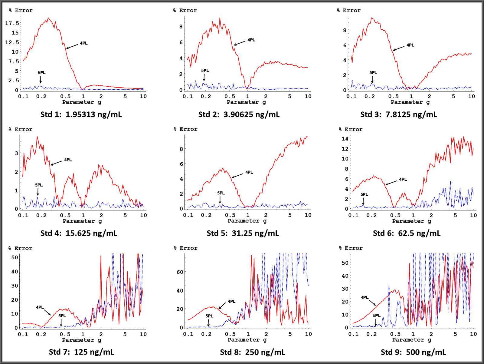
The graphs on the left depict the average backfit error (percent difference between the actual concentration and the computed concentration) from 200 simulated assays at each of 101 logarithmically equally-spaced values of coefficient g between 0.1 and 10 (the range most assay curves fall within). The other curve coefficients and weighting model were constrained to values typical for ELISA assays.
For each data set, the best fitting 5PL curve and the best fitting 4PL curve were determined. The mean of the computed concentrations for each standard were then determined from the 200 simulated curves at each of the 101 coefficient g curve models. The backfit error was then computed and plotted as a function of parameter g for each standard for both the 5PL and the 4PL curves. The results of this procedure are shown for each standard.
Except for the regions of the plots of Std 7, Std 8, and Std 9 where there is too much noise to draw any conclusions, these graphs show clearly that concentration estimates of the 5PL curve model are substantially more accurate than 4PL models when asymmetry is present. When there is no asymmetry present ( g = 1 ), the 5PL and 4PL error is identical, as one would expect. In practice, symmetrical curves are not usually observed.
In over 60,000 immunoassay and bioassay curves in our studies, 14% are symmetric with g between 0.9-1.1. In the 86% of the curves that are asymmetric, g is less than 0.3 in 21%, g is between 0.3-0.9 in 29%, g is between 1.2-10 in 23%, and g is greater than 10 in 13% of the total curves.
More information about these simulations and analysis can be found in the manuscript: The Five Parameter Logistic: A Characterization And Comparison With The Four Parameter Logistic. Further information on precision error and determining the limits of quantitation of assay curves can be found in the Tech Note: LOQs, LODs.
5PL (a>d) and 5PL (a<d) Forms
As noted above, 5PL curves can have 4 distinct functional forms, which are repeated in the table below:
The sign of b determines the direction of the slope of the 5PL function, and depends upon the order of a and d. Unlike 4PL curves, the order of a and d produce distinct functional shapes in 5PL curves. Most of the sigmoidal shapes that a 5PL can adopt can be formed by both 5PL (a>d) and 5PL (a<d) forms. However, sharp “knees” at transition zones occurring at the upper or lower shoulders of the curve can only be produced by one or the other 5PL form function.
5PL (a>d)
4PL
The 5PL (a>d) can form shapes with sharp transition knees at the upper shoulder (but not at the lower shoulder) as seen in the curve and residual graphs on the left above. The 5PL (a<d) can form shapes with sharp transition knees at the lower shoulder (but not at the upper shoulder) as seen in the curve and residual graphs on the left below. As can be observed in the matching 4PL curve and residual graphs to their right, the 4PL form cannot fit sharp transitions at either shoulder. In such cases where there is a sharp transition at the lower shoulder, STATLIA MATRIX automatically computes the 5PL (a<d) form. Otherwise the 5PL (a>d) form is used for 5PL curve fits.
5PL (a<d)
4PL
Numeric Fitting Algorithms for 5PL and 4PL Curves
There are two fundamental reasons that fitting algorithms sometimes fail to get the best 5PL fit: multiple local minima in the 5PL fitting function, and strong coupling between the coefficients of the 5PL function. Many fitting algorithms are handicapped by these problems, but the fitting algorithms in STATLIA MATRIX handle both issues.
In the 5PL fitting function, the sum of squares errors of the residuals often has more than one local minimum, i.e., a valley in the function’s values that is a local low point. Most numerical fitting algorithms will find the nearest local minimum to the starting guess of the fitting coefficients, in this case coefficients a, b, c, d, and g of the 5PL function. Without a good choice of the starting points, many algorithms get stuck in a sub-optimal local minimum which leads to a correspondingly worse fit than the global (MLE) minimum. STATLIA MATRIX uses several different algorithms to find the best starting point for the fitting algorithm.
The second issue is because certain subsets of coefficients of the 5PL function are strongly coupled. By adjusting them in tandem in the fitting algorithms, the 5PL curve can be made to appear nearly identical even though the values of the coefficients have changed dramatically. This problem can be minimized by having many dilutions that cover the entire range of the curve, but it can still occur. The problem is accentuated when less than the entire curve is covered by the dilution range. In other words, as the range of the data’s coverage of the curve becomes smaller, more subsets of coefficients become coupled. In mathematical terms, the fitting problem becomes ill-conditioned.
Coupled coefficients can lead to multiple local minima, it also can lead to regions in the 5D parameter space where the fitting function is nearly flat – so flat that many fitting algorithms stop because the flat region looks like a minimum. Quite often, such a region surrounds the entrance into the deep valley of the global minimum. If the fitting algorithm stops before it enters the deep valley, it can miss the global minimum completely, resulting in a fit that is worse than the actual global minimum (MLE).
STATLIA MATRIX uses sophisticated techniques to determine when it is truly at a minimum of the fitting function and avoids stopping too soon with a sub-optimal fit. It’s fitting algorithms also use various methods to avoid being trapped by flat regions that would cause them to iterate in infinite loops or to terminate due to lack of progress. These fitting algorithms allow the software to find the global minimum (MLE) when other software is unable. The 5PL fitting algorithms in STATLIA MATRIX have been used for many hundreds of thousands of asymmetric curve fits. For more information about fitting 5PL curves see the 5PL manuscript: The Five Parameter Logistic: A Characterization And Comparison With The Four Parameter Logistic.
Ease of Use in STATLIA MATRIX
Like all high precision tools, the engineering is incorporated inside so the user experience is simple, accurate and reliable. One of the key computations of all assays, whether an ELISA test, a potency bioassay, or a Tier 3 immunogenicity test, are the curve fitting computations. With STATLIA MATRIX, you get the best results possible in any analytical software plus the most informative graphs and metrics in the industry. Automatically.
All of the data from your assays are stored in the database, automatically. The weighting estimations are determined from your historical assays, after filtering outliers, automatically. The most powerful algorithms in the industry determine the best curve fits, automatically. Everything you need to know about these computations are presented to you in simple, easy to understand graphs only found in this software. Automatically.
The Pass/Fail acceptance criteria for the curve fit, and for the entire assay, is comprehensive yet flexible so it can be based on your SOP. The evaluation includes as much, or as little, detail as you want of the performance of your assay and its computations. Automatically.
The reports are detailed, or concise, in the format you want. All reports are stored and organized and always available. Automatically.
Setup is quick and intuitive. All of your instruments, PCs or VDIs, and LIM system are integrated seamlessly and raw data files, reagents and data are tracked automatically, so you can focus on running your assays.
STATLIA MATRIX is designed to provide a simple, yet powerful, enterprise workflow software system for all of the immunoassay, potency bioassay, and immunogenicity testing technologies in regulated laboratories.
REFERENCES
Bates DM, Watts DG. Nonlinear Regression Analysis and Its Applications. New York: Wiley, 1988.
Belanger BA, Davidian M, Giltinan DM The Effect of Variance Function Estimation on Nonlinear Calibration Inference in Immunoassay Data. Biometrics: 52, 158-175, 1996.
Boulanger B, Devanaryan V, Dewe W, Smith W. Statistical Considerations in Analytical Method Validation. Pharmaceutical Statistics Using SAS: A Practical Guide, 69-94, 2007.
Deming, SN. The 4PL: A Guide to the use of the four-parameter logistic model in bioassay. Statistical Designs, 2015.
DeSilva B, Smith W, Weiner R, Kelley M, Smolec J, Lee B, Khan M, Tacey R, Hill H, Celniker A. Recommendations for the Bioanalytical Method Validation of Ligand-binding Assays to Support Pharmacokinetic Assessments of Macromolecules. Pharmaceutical Research: 20 (11), 1885-1900, 2003.
Draper NR and Smith H. Applied Regression Analysis, 3rd Edition. New York: Wiley, 1998.
Dudley RA, Edwards P, Ekins, RP, Finney, DJ, McKenzie, IGM, Raab, GM, Rodbard, D; Rodgers RPC. Guidelines for Immunoassay Data Processing. Clinical Chemistry: 31 (8), 1264-1271, 1985.
Dunn JR, Wild D. Calibration Curve Fitting. The Immunoassay Handbook, Theory and Applications of Ligand Binding, ELISA and Related Techniques, 4th Edition, 323 – 336, 2013.
Fernandez AA, Stevenson GW, Abraham GE, Chiamori NY. Interrelations of the Various Mathematical Approaches to Radioimmunoassay. Clinical Chemistry: 29, 284-289, 1983.
Finney DJ. Response Curves for Immunoassay. Clinical Chemistry: 29 (10), 1762-1766, 1983.
Gottschalk PG, Dunn JR. Determining the Error of Dose Estimates and Minimum and Maximum Acceptable Concentrations from Assays with Nonlinear Dose-Response Curves. Computer Methods and Programs in Biomedicine, 204-215, 2005.
Gottschalk PG, Dunn JR. Measuring Parallelism, Linearity and Relative Potency in Immunoassay and Bioassay Data, Journal of Pharmaceutical Biostatistics 2005, 15 (3), 437–463.
Gottschalk PG, Dunn JR. The Five Parameter Logistic: A Characterization And Comparison With The Four Parameter Logistic. Analytical Biochemistry: 343, 54 – 65, 2005.
Press WH, Teukolsky SA, Vetterling WT, Flannery BP. Numerical Recipes, 3rd Edition. New York: Cambridge University Press, 2007.
Raab GM. Comparison of a Logistic and a Mass Action Curve for Radioimmunoassay Data. Clinical Chemistry 29: 1757-1761, 1983.
Seber GAF, Wild CJ. Nonlinear Regression. Hoboken NJ: Wiley, 2003.
www.brendan.com