RSSE (Chi-Square) Method and F Test Parallelism
The Direct Measure of Similarity Between Curves Is Used to Determine ParallelismSee your data in STATLIA MATRIX.
RSSE (Chi-Square) Method with Accurate Weighting Provides a Reliable and Stable Parallelism Method
The RSSE (Chi-Square) Method in Residual Parallelism is a direct measure of the similarity between the weighted residuals2 of the individual dilutions of the two curves. The RSSE (Chi-Square) Method measures the difference in the residual sum of squares error (RSSE) of unconstrained curves and curves constrained to the same shape to determine parallelism. When appropriately weighted (see the Tech Note: Curve Weighting), the difference in RSSEs beyond the constrained curves is a direct measure of the amount of nonparallelism between the two curves. A RSSE threshold can be established empirically for your test. Since this RSSE is a chi-square distributed value, a threshold for parallelism can also be set at a chi-square probability of your choice. This RSSE value, or its equivalent chi-square probability, sets a threshold for an acceptable amount of non-similarity between the two curves.
Without accurate weighting, the residual method can only be used as a hypothesis test with the F Test so that the weights are factored out. The F Test has known limitations of falsely failing some curve pairs when the curves are very good and falsely passing some curve pairs when the curves are very bad, but these issues are partially offset by the accurate weighting used by the software’s algorithms. STATLIA MATRIX automatically computes the F Test metrics for all residual parallelism comparisons.
STATLIA MATRIX’s Residual Parallelism can be used with 5PL, 4PL or linear regression, so you can use the model best suited to your data. You can also measure the parallelism and relative potency of more than one test sample in a single determination, so the relative potencies of multiple test samples can be measured relative to each other. See the manuscript: Measuring Parallelism, Linearity and Relative Potency in Immunoassay and Bioassay Data on the software’s residual parallelism method.

RSSE (Chi-Square) Method Example of Parallel Curves (Test Sample Same as Reference Standard)
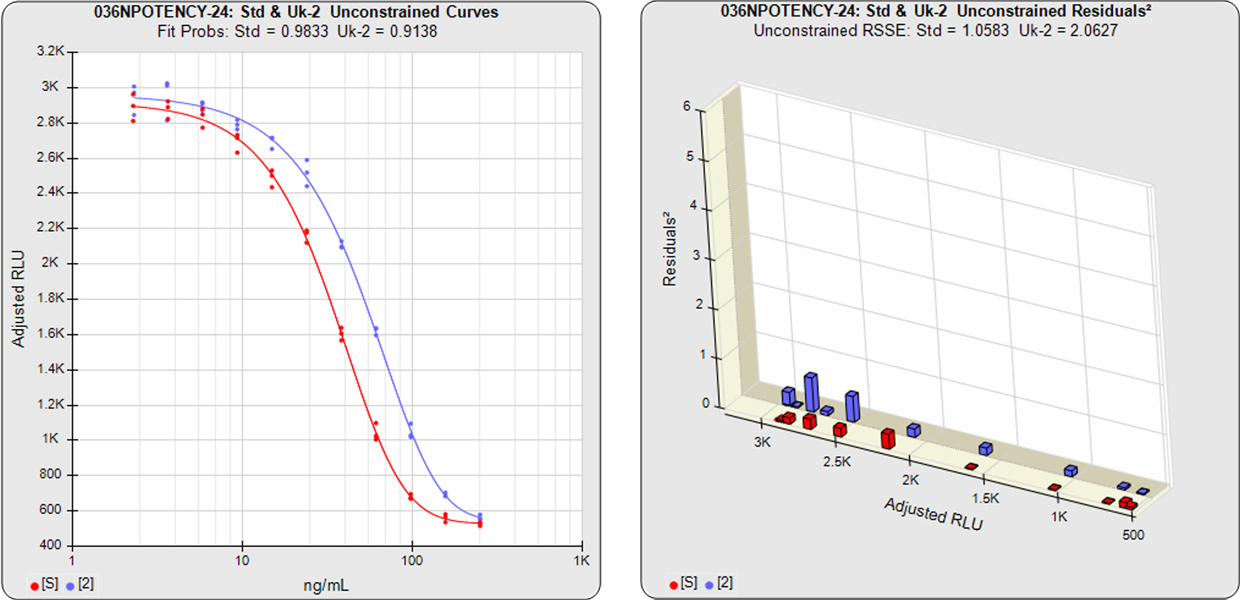
Unconstrained Curves
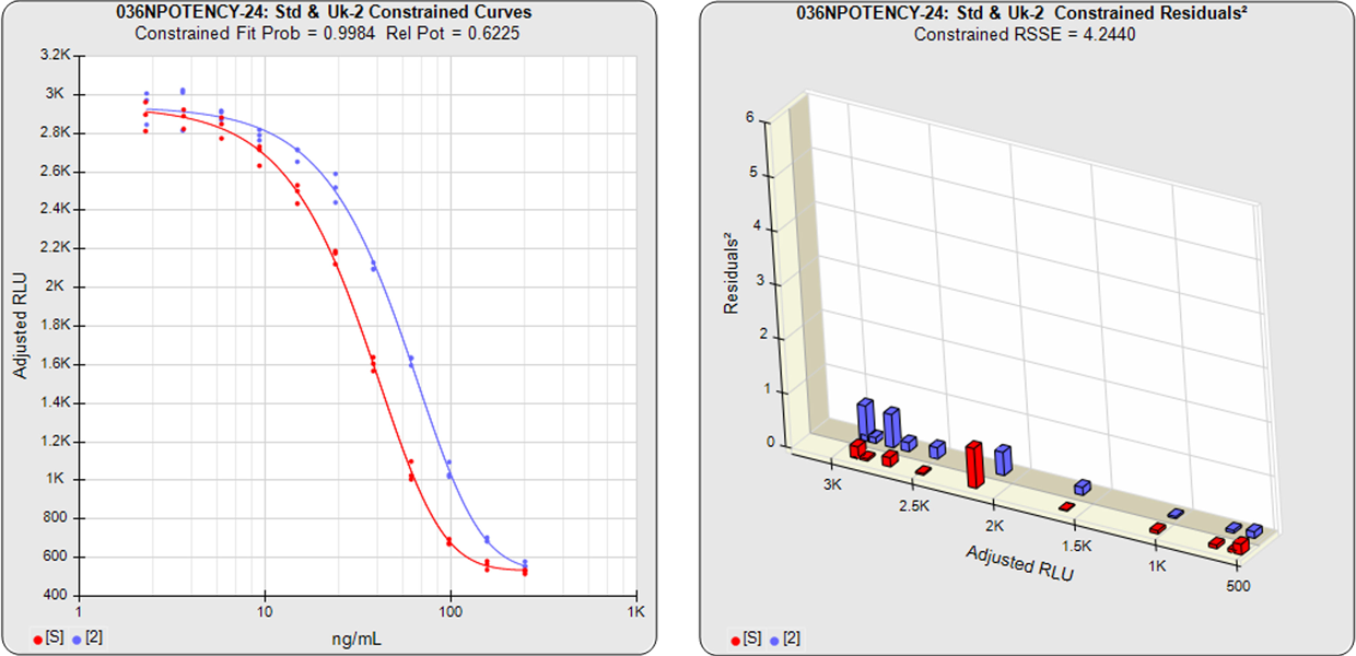
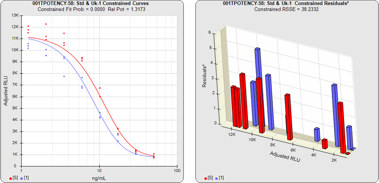
Constrained Curves
Residual2 Graphs Show the Fit of Each Dilution on the Curves
In the unconstrained curves, the data from both curves are computed using separate 5PL or 4PL curve fits. Linear regression can also be selected for linear data sets. The individual weighted residual sum of squares errors (RSSE) between each observed point and the curve is plotted on the weighted residuals2 graphs. The residual graph allows bad dilutions to be easily identified. There are no bad dilutions in this example. Since the unconstrained sample responses fit their curves separately, the RSSE’s are not affected by the amount of nonsimilarity (nonparallelism) between the curves.
With the constrained curves, the responses from both curves are forced to fit one identical curve shape that provides the best fit for both curves. Since the constrained curves use the same shape, the RSSE’s are affected by the amount of nonparallelism between the curves, and consequently have a higher RSSE than the unconstrained curves. In this example, the two samples generated similar dose response curve shapes, so the constrained curve was similar in shape to the two unconstrained curves and the difference between the unconstrained curves and the constrained curves is minimal.
Parallelism Determination
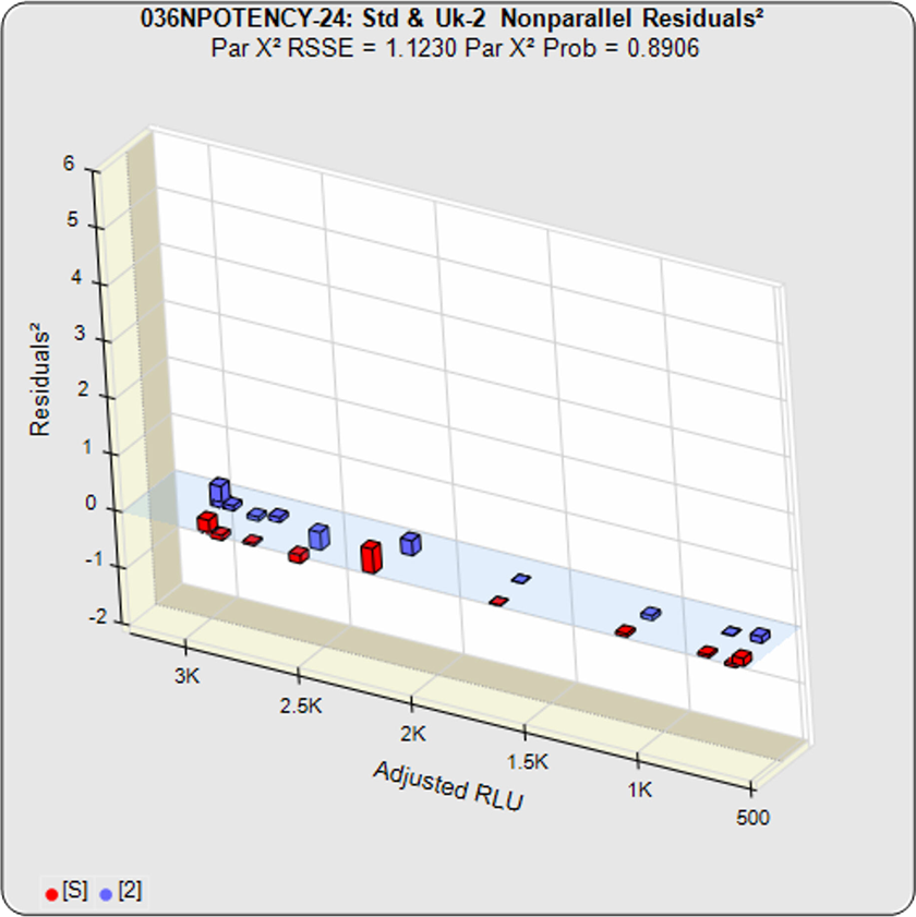
Because all of the residuals2 were appropriately weighted, the difference between the constrained RSSE and the unconstrained RSSE is a direct measure of the amount of nonparallelism between the two curves. This residuals graph shows the amount of nonparallelism between the individual dilutions.
The threshold for the nonparallel RSSE metric can be set to any value appropriate for your test. Since the nonparallel RSSE is chi-square distributed, parallelism can also be determined by a chi-square probability threshold of the RSSE (e.g. 0.01). Parallelism can also be determined from the F probability generated.
In this example, the two samples generated similar dose response curve shapes so the difference between the unconstrained curves and the constrained curves is minimal. Thus the nonparallel RSSE value is low (1.1230) and its equivalent chi-square probability is correspondingly high (0.8906). Therefore this test sample passes its parallelism test.
Relative Potency
The relative potency and its confidence limits are determined from the constrained curves. The relative potency in this example is 0.6225.
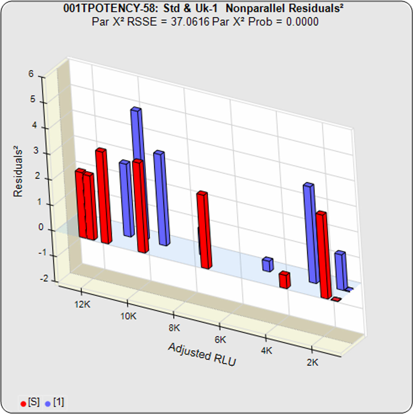
Nonparallel Residuals2
RSSE (Chi-Square) Method Example of Nonparallel Curves (Isomeric Impurity in Test Sample)
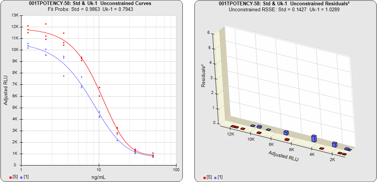
Unconstrained Curves
Constrained Curves
Residual2 Graphs Show the Fit of Each Dilution on the Curves
In the unconstrained curves, the data from both curves are computed using separate 5PL or 4PL curve fits. Linear regression can also be selected for linear data sets. The individual weighted residual sum of squares errors (RSSE) between each observed point and the curve is plotted on the weighted residuals2 graphs. The residual graph allows bad dilutions to be easily identified. There are no bad dilutions in this example. Since the unconstrained curves fit their mean responses separately, the RSSE’s are not affected by the amount of nonsimilarity (nonparallelism) between the curves. So these unconstrained curves have low RSSE values.
With the constrained curves, the responses from both curves are forced to fit one identical curve shape that provides the best fit for both curves. Since the constrained curves use the same shape, the RSSE’s are affected by the amount of nonparallelism between the curves, and consequently have a higher RSSE than the unconstrained curves. In this example, the two samples generated different dose response curve shapes, so the constrained curve was different in shape than the two unconstrained curves and the difference between the unconstrained curve and the constrained curve RSSEs is large.
Parallelism Determination
Because all of the residuals2 were accurately weighted, the difference between the constrained RSSE and the unconstrained RSSE is a direct measure of the amount of nonparallelism between the two curves. This residuals graph shows the lack of parallelism between the individual dilutions.
The threshold for the nonparallel RSSE metric can be set to any value appropriate for your test. Since the nonparallel RSSE is chi-square distributed, parallelism can also be determined by a chi-square probability threshold of the RSSE (e.g. 0.01). Parallelism can also be determined from the F probability generated.
In this example, the two samples generated different dose response curve shapes so the difference between the unconstrained curves and the constrained curves is large. Thus the nonparallel RSSE value is high (37.0616) and its equivalent chi-square probability is correspondingly low (<0.0000). Therefore this test sample fails its parallelism test.
Nonparallel Residuals2
Relative Potency
The relative potency and its confidence limits are determined from the constrained curves. Since the curves are not parallel, there is no meaningful relative potency between the reference standard and the test sample in this example.
Establish Your Parallelism Threshold From Your Previously Run Parallel Test Samples
Nonparallel Residuals2
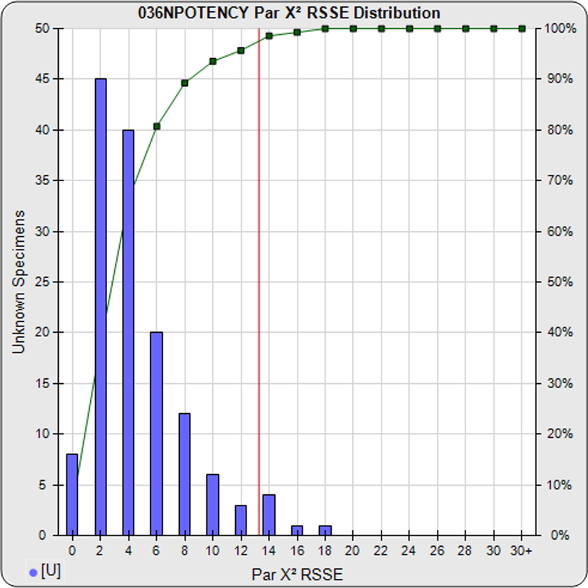
The parallelism threshold (red line) is computed from the nonparallel RSSE values from the unknowns (blue bars) in a pool of previously run assays, after masking curves with bad fits. The cumulative percentage of unknown specimens at each level of the RSSE nonparallel values is shown (in green). See the manuscript: Measuring Parallelism, Linearity and Relative Potency in Immunoassay and Bioassay Data on the software’s RSSE (Chi-Square) Method.
When appropriately weighted, these RSSE values are a direct measure of the amount of nonparallelism between the two curves. A RSSE threshold can be established empirically that includes an acceptable amount of non-similarity. The threshold can also be automatically computed by the software from your previous assays at a significance level appropriate for your test.
The development tools in STATLIA MATRIX can help you determine optimal dilution doses and other factors to make your potency test more stable and precise.
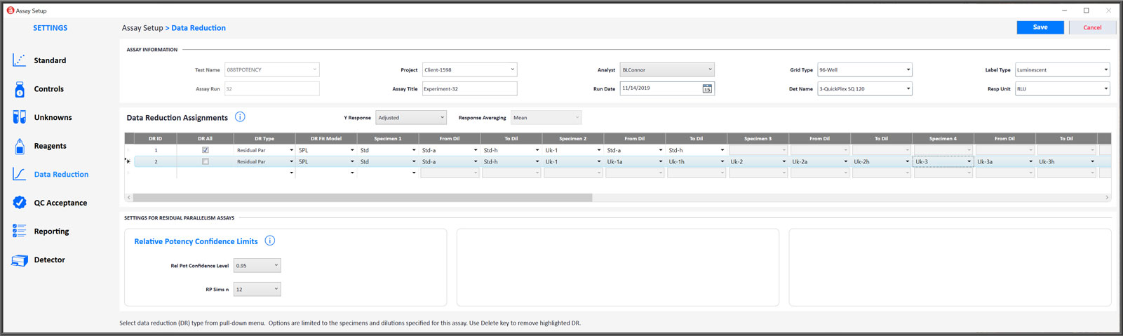
Modify Data Reduction Settings to Address Any Potency Assay Setup Requirement
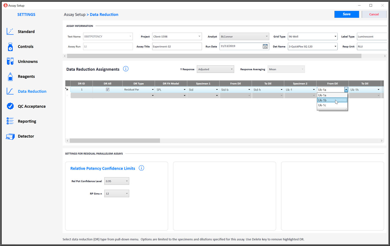
- You can select either the 5PL, 4PL or linear weighted regression curve fitting for RSSE (Chi-Square) Method and F Test assays.
- Both the RSSE (Chi-Square) Method and the F Test will be performed automatically for all test samples.
- End point hooks can be masked from the regression curve or line by starting and/or ending the dilution series at a different point.
- Check DR All to apply the same data reduction settings to all control and unknown dilution curves that have enough dilutions for the regression.
- The settings for computing the confidence limits for the relative potency can be adjusted.
Measure Multiple Test Samples Together or Multiple Data Reductions in the Same Assay
- You can measure the parallelism and relative potency of more than one test sample in a single determination with Residual Parallelism (RSSE (Chi-Square) Method or F Test) using the 5PL, 4PL or linear weighted regression curve fitting. Measuring multiple test samples together computes relative potencies relative to each other.
- You can set more than one data reduction for an assay. For example, you can compute separately determined relative potencies and the combined relative potencies above and compare the results.