Relative Potency and Parallelism In Potency Bioassays
Relative Potency Determination
The relative potency of a test sample is the amount of biological activity it produces compared to an equal amount of a reference standard under the same conditions. Relative potency is measured between a dilution series of doses from both materials. The responses from both dilution curves are constrained to fit regression curves having an identical curve shape that provides the best fit for both curves. The distance between the two curves on the log dose axis is the log of the relative potency, and its antilog is the relative potency. This relative potency is equivalent to the ratio of the IC50s between the two curves. Since the two curves are constrained to the same shape, all ICnn ratios will be the same as the IC50 ratio (e.g. black bars between the constrained curves in graph at right). Determining the relative potency from unconstrained curves is not as accurate since the two curves are never precisely the same shape and ICnn ratios will vary throughout the length of the curves.

Relative potency (black bars) of test sample (blue curve) compared to reference standard (red curve).
Confidence Limits of Relative Potency
An estimation of the confidence limits of the relative potency determination between the two dilution curves is required to measure its reliability and for averaging multiple independent determinations. The confidence limits of the relative potency from nonlinear curves can be determined using the Profile method, which estimates the asymptotic limits numerically, or the Monte Carlo method, which estimate the probability density limits from simulation estimates. The confidence limits of the relative potency from parallel lines can be determined using linear approximation.
Parallelism (Similarity) between Test Sample and Reference Standard
Testing for the similarity (parallelism) of the two regression curves obtained from each dilution series is a prerequisite for determining the relative potency of two bioactive substances in biological systems. When the two substances are not parallel (not similar), there is no meaningful relative potency between the reference standard and the test sample. Parallelism testing is also used for matrix effects (linearity), cross-reactivity, interfering substances, concentration estimation, and inhibition studies.
The dilution series can span a full dose response nonlinear curve or a more limited linear set of doses. The advantage of a full dose response curve is that some differences between substances only appear at high or low doses, and relative potency is more accurately determined. But the more limited number of doses needed for a linear comparison is an advantage for animal studies and requires simpler math computations.
The three main approaches to assessing the parallelism between substances are the RSSE (Chi-Square) method (a direct measure of parallelism), the F Test method (a hypothesis test), and Equivalence method (an empirical test). The first two methods utilize the residual (Residual Sum of Squares Error, RSSE) method from regression statistics (also called the Extra Sum of Squares method), and the latter method compares the confidence intervals of the regression coefficients. All of these methods are cited in the USP 1032, 1033, 1034 guidelines.
3 Methods for Determining Parallelism
RSSE (Chi-Square) Method for Parallelism
In regression statistics, the similarity of regressions (parallelism) is often determined with the Extra Sum of Squares method used in the RSSE (Chi-Square) and F Test methods. The RSSE (Chi-Square) method is a direct measure of the similarity between the weighted residuals2 of the individual dilutions of two regression curves (see manuscript: Determining Parallelism and Relative Potency in Immunoassay and Bioassay Data). This residual method, like the F Test method, can use any appropriately weighted least squares regression model (e.g. linear, 3PL, 4PL, 5PL) that provide an adequate fit to the dilution series data. One or both of the dilution series can be a partial dose-response curve. Residual methods are also effective with ill-behaved test methods because the weighting estimates match the test behavior. The RSSE method is sometimes called the Chi-Square method because the RSSEnonparallel result, like all appropriately weighted RSSEs, is chi-square distributed, and a chi-square probability of the RSSEnonparallel result can be used.
The RSSE (Chi-Square) method measures the difference in the residual sum of squares error (RSSE) of unconstrained (independent) curves (RSSEunconstrained) and curves constrained to the same shape (RSSEconstrained) to determine parallelism. When appropriately weighted for that test, the difference between the RSSEconstrained and the RSSEunconstrained is a direct measure (RSSEnonparallel) of the amount of non-parallelism between the assayed data points of the two curves. This RSSEnonparallel result becomes progressively larger the more nonparallel the two curves are.
Unconstrained Curves

Constrained Curves

Standard and Test Sample
Residuals2 (RSSEunconstrained)
Standard and Test Sample
Residuals2 (RSSEconstrained)
A RSSE threshold can be established empirically that includes an acceptable amount of nonsimilarity for that test. Since the differences between the residuals of each assayed data point are measured individually, the RSSEnonpar allows individual dose regions to be examined. This can be an important benefit because some differences between the test sample and the reference standard only appear at high or low doses.
Importance of Weighting for Parallelism Tests
Statistical curve fitting uses a method called least squares regression fitting, which derives the one set of coefficients that has the smallest sum of squared residuals (RSSE) for that curve model. A squared residual is the vertical distance between the observed point and the curve, squared, divided by the estimated variance at that point. Weighting the squared residual errors with their estimated variances normalizes each point and allows all the points to contribute equally to the regression curve. Accurately estimated variances of the data points are necessary to obtain the Maximum Likelihood Estimate (MLE) of the true underlying regression curve. Adequate weighting can be determined from a single assay, but more accurate weighting estimates are obtained from the responses of pooled assays (see the Tech Note: Curve Weighting). Accurately weighted residuals are necessary for the RSSE (Chi-Square) method but not for the F Test method. However, accurate weighting of the F Test regressions partially offset the issues observed with very good and very poor curve fits.
Unconstrained Curves and Constrained Curves
In the unconstrained curves on the left in the graphs above, the data from both curves are computed independently using separate (5PL) curve fits. The individual weighted residuals2 between each observed point and its respective curve are plotted on the weighted residuals2 graphs next to the curves. The sum of these weighted residuals2 is the RSSEunconstrained. Since the unconstrained sample responses fit their curves independently, the RSSE’s are not affected by any nonsimilarity (nonparallelism) between the curves.
With the constrained curves on the right in the graphs above, the responses from both curves are forced to fit one identical curve shape that provides the best fit for both curves. Since the constrained curves both use the same shape, the RSSEconstrained is affected by the amount of nonsimilarity between the two curves, and consequently have a higher RSSE than the unconstrained curves.
RSSE(Chi-Square) Method Provides Direct Measure of Similarity Between Curves

The difference between the RSSEconstrained and the RSSEunconstrained shown above is a direct measure of the amount of nonsimilarity (RSSEnonparallel) between the two curves. In this example, the two materials tested were the same material so the RSSEnonparallel result is minimal. The parallelism threshold for the RSSEnonparallel result can be set to include any amount of nonsimilarity appropriate for your test.
Parallel and Nonparallel Test Samples
In the examples below, two test samples from the same assay were each compared to the same reference standard from that assay.
Example 1
In the first example, the test sample was a control having the same material as the reference standard. A 5PL curve was fit to both curves in the unconstrained and constrained fits. The RSSEunconstrained shows good fits for each independently fit curve. Because the two materials were the same, their constrained shapes were very similar to their unconstrained shapes and the RSSEnonparallel result was minimal.
Unconstrained Curves

Constrained Curves

Standard and Test Sample
Residuals2 (RSSEunconstrained)
Standard and Test Sample
Residuals2 (RSSEconstrained)
Constrained – Unconstrained
RSSEnonparallel Residuals2
Example 2
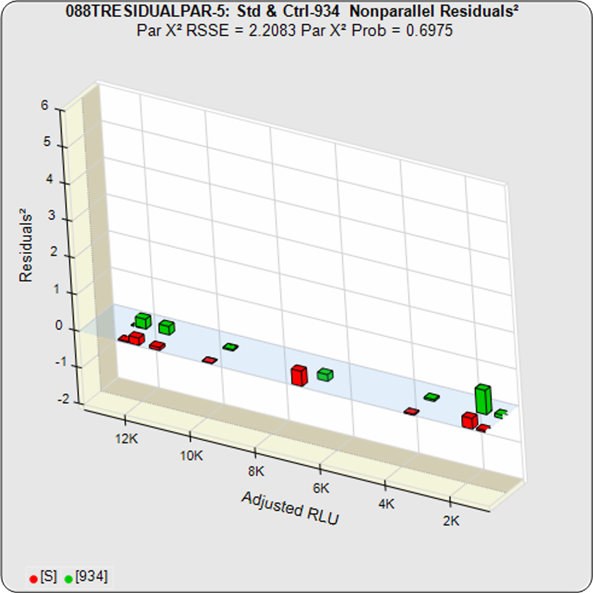
In the second example from the same assay, the test sample had an isomeric impurity that affected the biological reaction. The RSSEunconstrained shows good fits for each independently fit curve. As a result of the two materials not being the same, their constrained shapes were not similar to their unconstrained shapes and the RSSEnonparallel result was large. It can also be observed from the nonparallel residuals² of the individual doses that the effect of the isomeric impurity was more pronounced in the lower doses. Since the curves are not parallel, there is no meaningful relative potency between the reference standard and this test sample.
Unconstrained Curves

Constrained Curves

Standard and Test Sample
Residuals2 (RSSEunconstrained)
Standard and Test Sample
Residuals2 (RSSEconstrained)
Constrained – Unconstrained

RSSEnonparallel Residuals2
Determining a Parallelism Threshold Empirically for RSSE (Chi-Square) Method
A RSSE parallelism threshold can be determined empirically from previous assays that include test samples that have acceptable amounts of nonsimilarity appropriate for your test, as illustrated in the frequency histogram shown below. The cumulative percentage of test samples at each level of RSSEnonparallel results is also plotted. A chi-square probability of the RSSEnonparallel result at an appropriate significance level can also be set as an a priori threshold (e.g. 0.01) for initial tests, as illustrated by the solid red line. The limit can also be set empirically to include an acceptable amount of non-similarity, as illustrated by the dashed red line.
RSSEnonparallel Parallelism Threshold

Threshold computed at .99 confidence limit of RSSEnonparallel results from pooled test samples (solid red line), or set empirically with acceptable amount of non-similarity (dashed red line).
F Test Method for Parallelism
The other residual method used in regression statistics to determine parallelism is the F Test method. Like the RSSE (Chi-Square) method, the F Test method uses the RSSEnonparallel and RSSEunconstrained from the RSSE (Chi-Square) method. However, it then computes a ratio of the RSSEnonparallel / RSSEunconstrained and determines an F probability from that ratio (shown below). A null hypothesis that there is no statistical difference in similarity between the two curves is tested, typically at 0.05 significance. The popularity of the F Test method is that it allows any least squares regression model with full or partial dilution series curves without having accurate weighting models. A single estimated variance obtained from all replicate responses is used to compute the residuals², so it is more reliable when a fairly narrow range of responses are used. A known weakness of the F Test method is that the very small RSSEunconstrained from very good curve fits will fail parallel curves and the very large RSSEunconstrained from very bad curve fits will pass nonparallel curves.
F Test Method

Equivalence Method for Parallelism
The Equivalence method (or Confidence Interval Parallelism) is a measure of the similarity between the asymptotic end points plus the slope of the inflection point of two 4PL curves or the slopes of two lines. Since finding the joint confidence interval for nonlinear regressions is an unsolved problem, the Equivalence method estimates the confidence intervals of each coefficient as a separate determination. The Equivalence method compares the confidence interval limit deltas of the test sample and reference standard A, B, and D coefficients of 4PL curves or the B coefficient of linear regressions. The confidence interval limits can be determined using the Profile method which estimates the asymptotic limits numerically, the Monte Carlo method which estimate the probability density limits from simulation estimates, or linear approximation. The deltas are either the ratio or differences between the upper limits of each and the lower limits of each (see illustration at right). The deltas must all fit within defined goalpost borders to be considered parallel. Goalpost borders are established using empirical data from parallel and nonparallel curve pairs.

Confidence interval limit deltas for 4PL curve coefficients A, B and D
In the two examples below, the parallel and nonparallel test samples from the assay shown in the RSSE (Chi-Square) method examples above were reexamined using the Equivalence Method. The unconstrained curves and weighted residuals2 of the reference standard and test sample are shown in the first two graphs for each test sample. As can be seen in the residual graphs, all of the dilution curves had acceptable individual fits.
For the Equivalence method, the ratio (or difference) of the low confidence interval limits of the test sample and reference standard are calculated, and the ratio (or difference) of their upper limits are calculated for each curve coefficient. The equivalence chart to the right of the curves and residuals show the lower and upper confidence interval limit ratios as horizontal bars between them for the A, B and D 4PL curve coefficients. The goalpost borders, determined empirically as discussed below, are shown as blue vertical bars. In these examples, the horizontal bars are green when completely inside blue goalpost borders (Pass) and red when any part of the interval is outside the goalpost borders (Fail).

Unconstrained Curves and Residuals2 (RSSEunconstrained)
Example 1
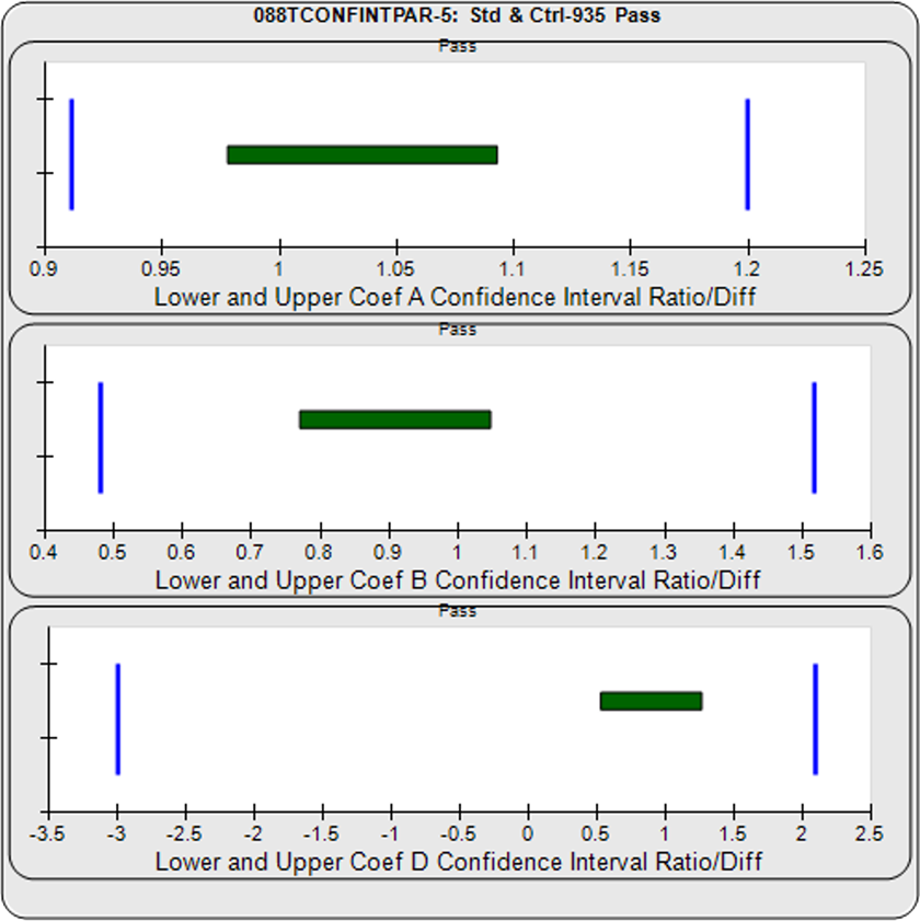
Equivalence Chart
The first control test sample in Example 1 having the same material as the reference standard, all of the coefficient deltas were within their respective goalpost borders and the test sample passed its parallelism determination. In the second test sample in Example 2, which had an isomeric impurity, the upper asymptote A coefficient was partially outside its goalpost delta so that test sample failed its parallelism determination.

Unconstrained Curves and Residuals2 (RSSEunconstrained)
Example 2

Equivalence Chart
Determining Goalpost Borders Empirically for Equivalence Method
Equivalence goalpost borders for the lower and upper confidence interval limits can be determined empirically from previous assay test samples that have acceptable similarity. Separate lower and upper goalpost borders are established for each curve coefficient. In graph below, the ratios of the lower and upper confidence interval limits from 140 reference standard and test sample pairs are displayed as green vertical lines. Goalpost borders (blue bars) can be computed as a percentile limit or other statistical determination from pooled assay results, or set at goalpost borders established by the laboratory.
Equivalence Goalpost Borders

140 Confidence Interval Ratios
Combining Relative Potency Results
Three methods are cited in USP 1034 guidelines for combining multiple determinations of the relative potency of a test sample from independent assays to establish a reportable potency and 95% confidence intervals.
Combined relative potency results can be determined from a simple arithmetic mean (A) and confidence limits from the relative potency determinations, from a geometric mean (G) and confidence limits of the antilog of the logarithms of the determinations, or from a weighted mean (W) computed from the logarithms of the determinations weighted by the log of the high/low confidence limits of each relative potency determination distributed as a homogeneous or heterogenous population.

Combined Single Assay Relative Potencies
The parallelism and relative potency of more than one test sample in a single assay can be determined from a single constrained 5PL, 4PL, 3PL or linear curve shape computed from the reference standard and all of the test samples (see graph below) with the residual methods (RSSE (Chi-Square) and F Test ). Measuring multiple test samples together from a single constrained curve computes all of the relative potencies relative to each other.
Combined Single Assay Relative Potencies
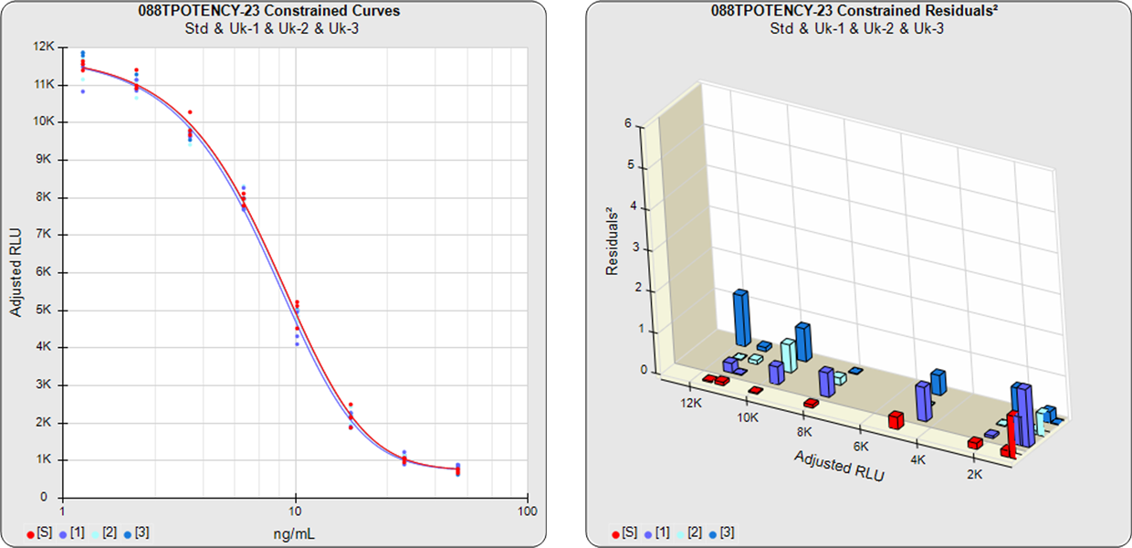
Constrained Curves and Residuals² (RSSEconstrained)
REFERENCES
Bates DM, Watts DG. Nonlinear Regression Analysis and Its Applications. New York: Wiley, 1988.
Belanger BA, Davidian M, Giltinan DM The Effect of Variance Function Estimation on Nonlinear Calibration Inference in Immunoassay Data. Biometrics: 52, 158-175, 1996.
Boulanger B, Devanaryan V, Dewe W, Smith W. Statistical Considerations in Analytical Method Validation. Pharmaceutical Statistics Using SAS: A Practical Guide, 69-94, 2007.
Deming, SN. The 4PL: A Guide to the use of the four-parameter logistic model in bioassay. Statistical Designs, 2015.
Draper NR and Smith H. Applied Regression Analysis, 3rd Edition. New York: Wiley, 1998.
Dunn JR, Wild D. Calibration Curve Fitting. The Immunoassay Handbook, Theory and Applications of Ligand Binding, ELISA and Related Techniques, 4th Edition, 323 – 336, 2013.
Finney DL, Phillips P. The Form and Estimation of a Variance Function, with Particular Reference to Immunoassay. Applied Statistics 26, 312-320 (1977).
Finney DJ. Statistical Methods in Biological Assays, 3rd Edition, London: Charles Griffin (1978).
Gottschalk PG, Dunn JR. Determining the Error of Dose Estimates and Minimum and Maximum Acceptable Concentrations from Assays with Nonlinear Dose-Response Curves. Computer Methods and Programs in Biomedicine, 204-215, 2005.
Gottschalk PG, Dunn JR. Measuring Parallelism, Linearity and Relative Potency in Immunoassay and Bioassay Data, Journal of Pharmaceutical Biostatistics 2005, 15 (3), 437–463.
Gottschalk PG, Dunn JR. The Five Parameter Logistic: A Characterization And Comparison With The Four Parameter Logistic. Analytical Biochemistry: 343, 54 – 65, 2005.
Jonkman JF, Sidik K. Equivalence Testing for Parallelism in the Four- Parameter Logistic Model. J. Biopharm. Stat. 19, 2009: 818–837.
Liu JS. Monte Carlo Strategies in Scientific Computing. New York: Springer, 2004.
Seber GAF, Wild CJ. Nonlinear Regression. Hoboken NJ: Wiley, 2003.
Singer R, Lansky DM, Hauck WW. Bioassay Glossary. Stimuli to the Revision Process. Pharmacopeial Forum 32, 2006: 1359–1365.
USP Chapter <1032> Design and Development of Biological Assays. USP Pharmacopeial Convention: Rockville, MD, 2013.
USP Chapter <1033> Biological Assay Validation. USP Pharmacopeial Convention: Rockville, MD, 2013.
USP Chapter <1034> Analysis of Biological Assays. US Pharmacopeial Convention: Rockville, MD, 2013.
Yang H, Kim HJ, Zhang L, Strouse RJ, Schenerman M, Xu-Rong J. Implementation of Parallelism Testing for Four Logistic Model in Bioassays. PDA J. Pharm. Sci. Technol. 66, 2012: 262–269.
www.brendan.com