Weighting In Logistic Curve Regressions

FDA and European Pharmacopeia guidelines specify appropriate weighting of responses with their estimated variances (i.e., the squared residuals) for all immunoassay and bioassay regression curves. A squared residual is the vertical distance between the observed point and the curve, squared, divided by the estimated variance at that point. Weighting is specified because of the substantial effect weighting has on the sensitivity, reliability and accuracy of the results. Accurate weighting used with an appropriate curve fitting model can increase the reportable range of an assay. Other analytical computations that require accurate weighting include measuring the parallelism and relative potency between curves in potency tests, precision profiles of concentration error, limits of quantitation and detection, confidence limits around parameters, sample replicate precision, and identifying precision and residual outliers.

Heteroscedasticity of Variances Between Dilutions

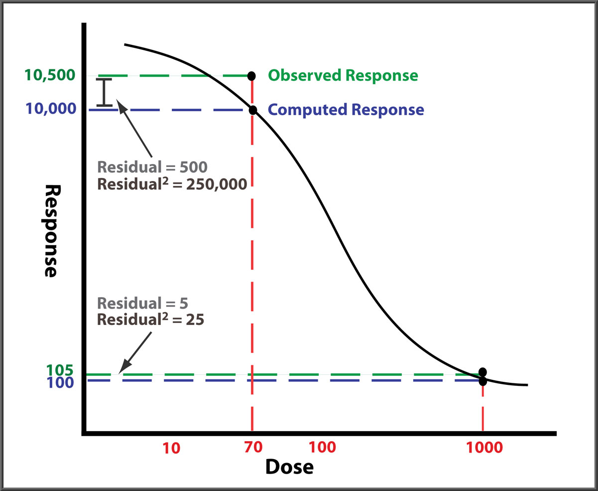
Responses can differ by two or more orders of magnitude between end points, and their response variances (residuals²) can differ by more than four orders of magnitude. In this illustration (not drawn to scale), both observed responses are 5% higher than the curve. But the squared error (residual²) of the high response point dwarfs that of the low response point. Without weighting each response with the inverse of its expected variance (residual²), the curve will be fitted predominantly to the high responses with little influence from the low responses because that will yield the regression with the lowest sum of residuals² (RSSE, residual sum of squares error). However, accurately weighting each response with its estimated variance ensures that all dilution points contribute equally to the final regression curve.

An accurate weighting regression of the response variance models the two sources of error, the dilutional variance and the residual error.

DILUTIONAL VARIANCE

Dilutional variance can be estimated from the replicate variances of each dilution. The dilutional variance contains the signal error from the detector, the systemic intra-assay error from the kinetic reactions, pipetting, reagents, incubation conditions, reactive phase separation, and random error. A dilutional variance estimate can be made from one assay, but more reliable variance estimates are obtained from a pool of 6 or more historical assays using the error mean sum of squares from an analysis of variance (ANOVA) of each dilution.  Pooled assays provide a larger sample size to determine a reliable estimate of the true variances in a test method. The responses and their variances are fitted to the well documented power regression (log responses, log variances), which reduces the heteroscedasticity, or change, of the variances. This generates a variance regression in the form AY^B, where A is the error term, Y is the response, and B is the heteroscedasticity in the variances across dilutions. The error term A can vary from 10^-6 to 10⁴ and the heteroscedascity term B can vary from 0.5 to 3 between different test methods and different label types. The fixed weighting equations 1/Y and 1/Y² are this formula, with A = 1 and B = 1 and 2, respectively.

RESIDUAL ERROR

Residual error is the imprecision of the individual dilution concentrations plus the lack of fit error of the curve model in each assay. The residual error of 4PL regressions is usually greater than that of 5PL regressions when the curves are asymmetric in shape. Like the dilutional variance, a residual error estimate can be made from one assay, but a more reliable estimate is obtained from a pool of 6 or more historical assays. This residual error is added to the dilutional variance error (A) for the final weighting regression of the response variances. In the study shown at the end of this Tech Note, the residual error from 5PL curves computed from 164 test methods had a median value of 6% of A, and the residual error from 4PL curves from the same tests had a median value of 34% of A.

Accurate Weighting from Pooled Assays

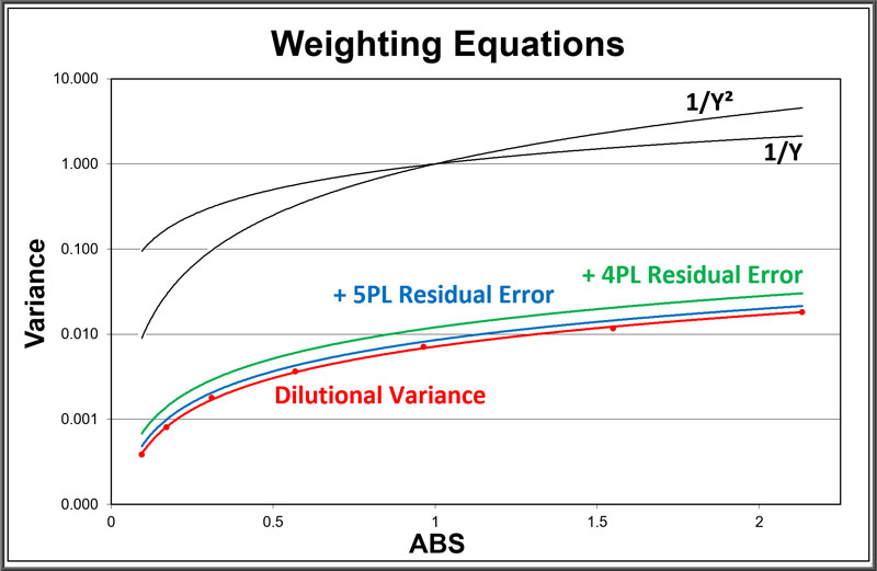
The dilutional variance power regression (red) models the average variance of each standard dilution (red dots) from an ANOVA of pooled assays. The residual error from 5PL curves (blue) and 4PL curves (green) of the same pooled assays are added to the dilutional variance regression.

As often noted in the literature, deriving the weighting from pooled assays is the best way to obtain accurate weights for immunoassay and bioassay dilution curves. The weighting regressions for these same pooled assays using a variance of Y (weight = 1/Y) and Y² (weight = 1/Y²) for each dilution response are plotted in black. These fixed regressions show how much these weighting models can differ from pooled weighting.

Weighting Model

In the study shown below, 6, 12, 20, or 30 assays were pooled by test for 164 immunoassay (LBA) and potency tests to determine their individual test weighting models.  In these tests, coefficient A varied from from 10^-5 to 10⁴ and coefficient B varied from 0.2 to 3 between the different test methods and different label types, as shown in the graphs below.  The label types included colorimetric OD (88), fluorescent FL (33), luminescent RLU (24) and isotopic CPM (19) labels.

In regression statistics, an accurately weighted RSSE is a chi-square distributed value whose average from a pool of assay curves equals the degrees of freedom (number of points – number of parameters). The RSSEs from the individual assay curves from these 164 tests, computed with their respective weighting regressions, were then averaged for each test.  The pooled RSSEs averages for each test were within 5% of their respective degrees of freedom, as predicted in regression statistics when accurate variance estimations are used.

Note that the RSSE of a curve regression can be expressed as a chi-square probability (Fit Prob) to simplify the evaluation of how well the curve fit the data. And since the variability of the test method is incorporated into the weighting, the Fit Prob is equally appropriate for well-behaved tests and ill-behaved test methods.

Weighting Variance = 1 / AY^B

Weighting Results

The ELISA assay shown in the graphs below had 6 standard dilutions with doses ranged from 0.3 (Std-a) – 3000 (Std-f) ng/mL.   A 5PL curve was computed using pooled weighting estimates (A=0.0007, B=1.6597) for the response variances and an unweighted (A=1, B=0) 5PL was also computed using the same data.  The weighted and unweighted 5PL curves are shown next to graphs showing the %Bias backfit of the computed dilution concentrations compared to their actual concentrations.

In the weighted 5PL, each dilution response is weighted with its own estimated variance so all points contribute equally to the final regression solution.  But in unweighted regressions the curve is fitted predominantly to the high responses with little influence from the low responses (as described above).  While scaling effects in semi-log standard curve graphs often make the low end appear to be a “good” fit, the backfit concentrations of the low responses show how much %Bias error can result from unweighted regressions at those doses.

Unweighted 5PL Curve

The ELISA assay shown in the graphs above illustrate the importance of accurate weighting on the reliability of concentration results at the low end. Weighting is also important particularly at the low end when examining the parallelism and relative potency of curves in potency tests.

For more information on weighting 5PL and 4PL curves, see the Tech Note at: www.Brendan.com/5pl-curve-fitting. To see how weighting is used for limits of quantitation (LOQ) and limits of detection (LOD), see the Tech Note at: www.Brendan.com/loqs-lods. For more information on the studies referenced above contact sales@brendan.com.

REFERENCES

Belanger BA, Davidian M, Giltinan DM  The Effect of Variance Function Estimation on Nonlinear Calibration Inference in Immunoassay Data.  Biometrics: 52, 158-175, 1996.

Davidian M, Carroll R.J., Smith W. Variance Functions and the Minimum Detectable Concentration in Assays. Biometrika 1988, 75, 549–556.

DeSilva B, Smith W, Weiner R, Kelley M, Smolec J, Lee B, Khan M, Tacey R, Hill H, Celniker A. Recommendations for the Bioanalytical Method Validation of Ligand-binding Assays to Support Pharmacokinetic Assessments of Macromolecules. Pharmaceutical Research 2003, 20 (11), 1885-1900.

Dudley R.A., Edwards P, Ekins, R.P., Finney, D.J., McKenzie, I.G.M., Raab, G.M., Rodbard, D; Rodgers R.P.C. Guidelines for Immunoassay Data Processing. Clinical Chemistry 1985, 31 (8), 1264-1271.

Dunn JR, Wild D.  Calibration Curve Fitting. The Immunoassay Handbook, Theory and Applications of Ligand Binding, ELISA and Related Techniques, 4th Edition, 323–336, 2013.

European Pharmacopeia 5.3. Statistical Analysis of Results of Biological Assays and Tests 2003, 4375-4406.

Finney D.J. Response Curves for Immunoassay. Clinical Chemistry 1983, 29 (10), 1762-1766.

Gottschalk PG, Dunn JR. Determining the Error of Dose Estimates and Minimum and Maximum Acceptable Concentrations from Assays with Nonlinear Dose-Response Curves.  Computer Methods and Programs in Biomedicine, 204-215, 2005.

Gottschalk PG, Dunn JR. Measuring Parallelism, Linearity and Relative Potency in Immunoassay and Bioassay Data, Journal of Pharmaceutical Biostatistics 2005, 15 (3), 437–463.

Gottschalk PG, Dunn JR.  The Five Parameter Logistic: A Characterization And Comparison With The Four Parameter Logistic.  Analytical Biochemistry: 343, 54–65, 2005.

Raab, G.M. Estimation of a Variance Function, with Application to Immunoassay. Applied Statistics 1981, 3 (1), 32-40.

U.S. Department of Health and Human Services, Food and Drug Administration, Center for Drug Evaluation and Research (CDER), Center for Veterinary Medicine (CVM). Bioanalytical Method Validation, Guidance for industry. Biopharmaceutics, May 2018.

www.brendan.com